Lightweight Neural Gravitational-Wave Detection 2026

Resources: Paper | GitHub

Implementation: Python with PyTorch/PyTorch Lightning; trained and evaluated on real LIGO data from the Gravitational Wave Open Science Center (GWOSC).

Overview:

This project studies how to build small neural networks that can detect gravitational waves (GW) reliably in real LIGO noise. The difficulty in gravitational wave detection is that true gravitational-wave signals are rare and often weak compared with the non-stationary, glitchy detector noise they are embedded in. Rather than focusing only on the network architecture, I looked at the complete detection pipeline: how training examples are constructed, how the detector streams are whitened and normalized, what signal strengths the model sees during training, how model outputs are converted into triggers, and how stable the results are across changing detector conditions and independent training runs.

The work grew out of my original AttenGW detector. While fine-tuning that system, I found that pipeline design choices often mattered more than making the architecture itself more complicated. That eventually turned into a larger architecture and pipeline study.

Models & Pipeline:

I compared twelve lightweight architectures, including temporal convolutional networks (TCNs), hierarchical dilated convolutional networks, cross-attention and graph models, temporal attention, a time-frequency model, ResNet, and bidirectional Mamba. Under the training setup tested here, the TCN variants were consistently among the strongest models. Since several of them performed similarly, I selected the simplest one, an early-fusion TCN that combines Hanford and Livingston at the input, for the final evaluation.

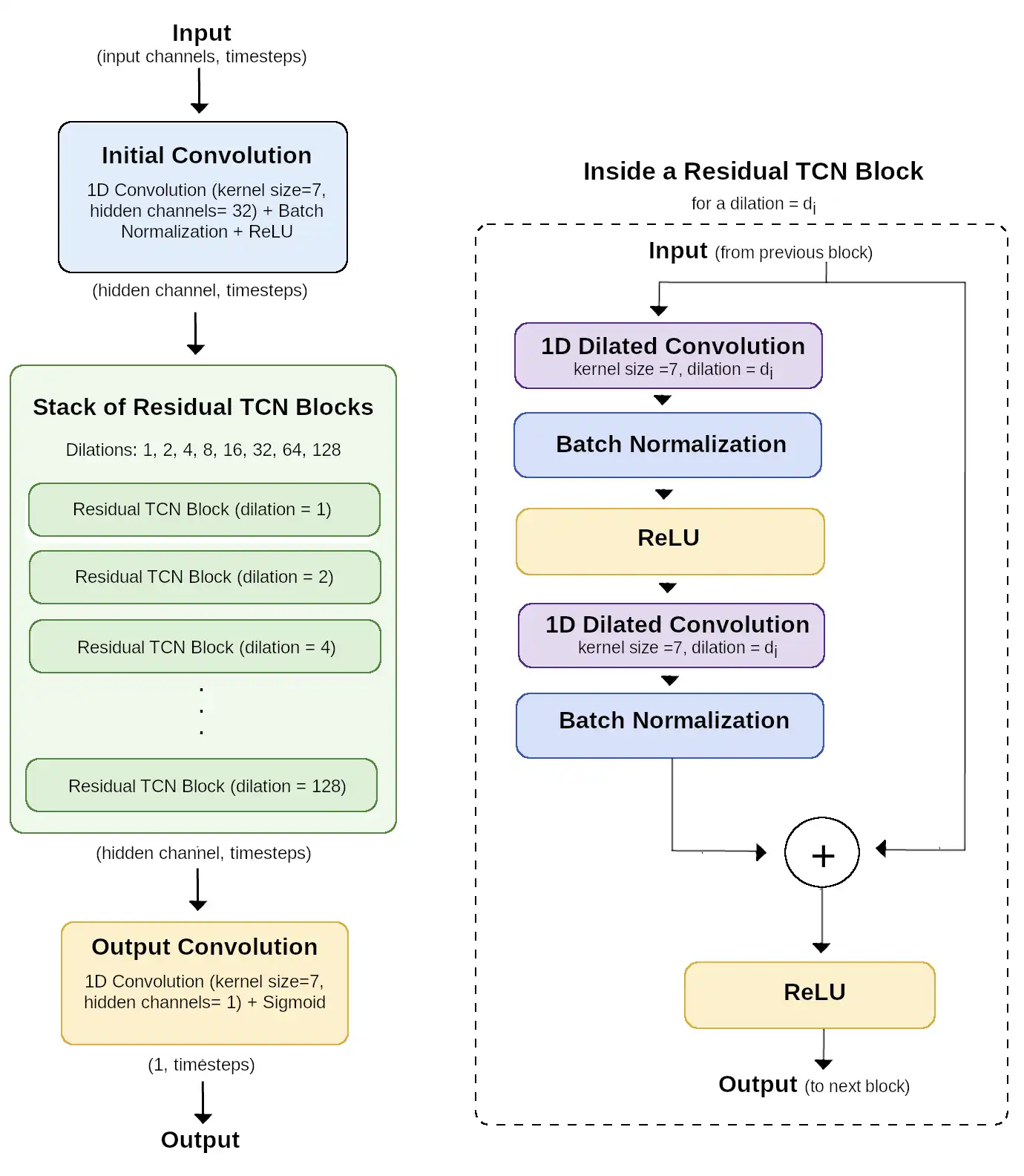
Schematic of the lightweight early-fusion temporal convolutional network used for gravitational-wave detection.

Figure 1. The 116k-parameter early-fusion TCN used for the final evaluation. Hanford and Livingston are combined at the input and processed jointly through dilated temporal convolutional blocks.

I ran a series of ablations around the network. Among the choices that improved the final pipeline were shared normalization across the two detectors (which singinficantly improved seed-to-seed variation but had a smaller impact on per-seed performance), an 8 s whitening context, training on a SNR curriculum that includes signals below the eventual detection limit, and retaining a representative amount of non-stationary detector noise rather than filtering the training set too aggressively. Trigger construction also became simpler: a smoothed maximum of the model output performed better than the more complicated peak-height, width, and plateau criteria used in the earlier AttenGW pipeline.

I also introduced an ASD-mismatch diagnostic to quantify how different the detector noise at evaluation time is from the noise seen during training. For each evaluation segment, the metric compares its amplitude spectral density (ASD) with the training-noise ASDs and measures how far it lies from the k most similar training examples. A low mismatch therefore means that the evaluation noise looks spectrally similar to conditions represented in the training set, while a high mismatch indicates a more unfamiliar noise environment.

d_ASD(s) = exp[ 1/k ∑_{t ∈ N_k(s)} d(s,t) ]

d(s,t) = 1/N_f ∑_i=1^N_f |x_s(f_i) − x_t(f_i)|

Here, s is an evaluation segment and t is a training segment. x_s(f_i) is the log-ASD of segment s at frequency bin f_i, N_f is the number of frequency bins, and N_k(s) denotes the k most similar training segments to s. This gives a model-independent way to separate evaluation data into low-, medium-, and high-mismatch regimes and test how robust a detector is as the noise distribution changes. Across the models tested, sensitivity generally decreased as ASD mismatch increased.

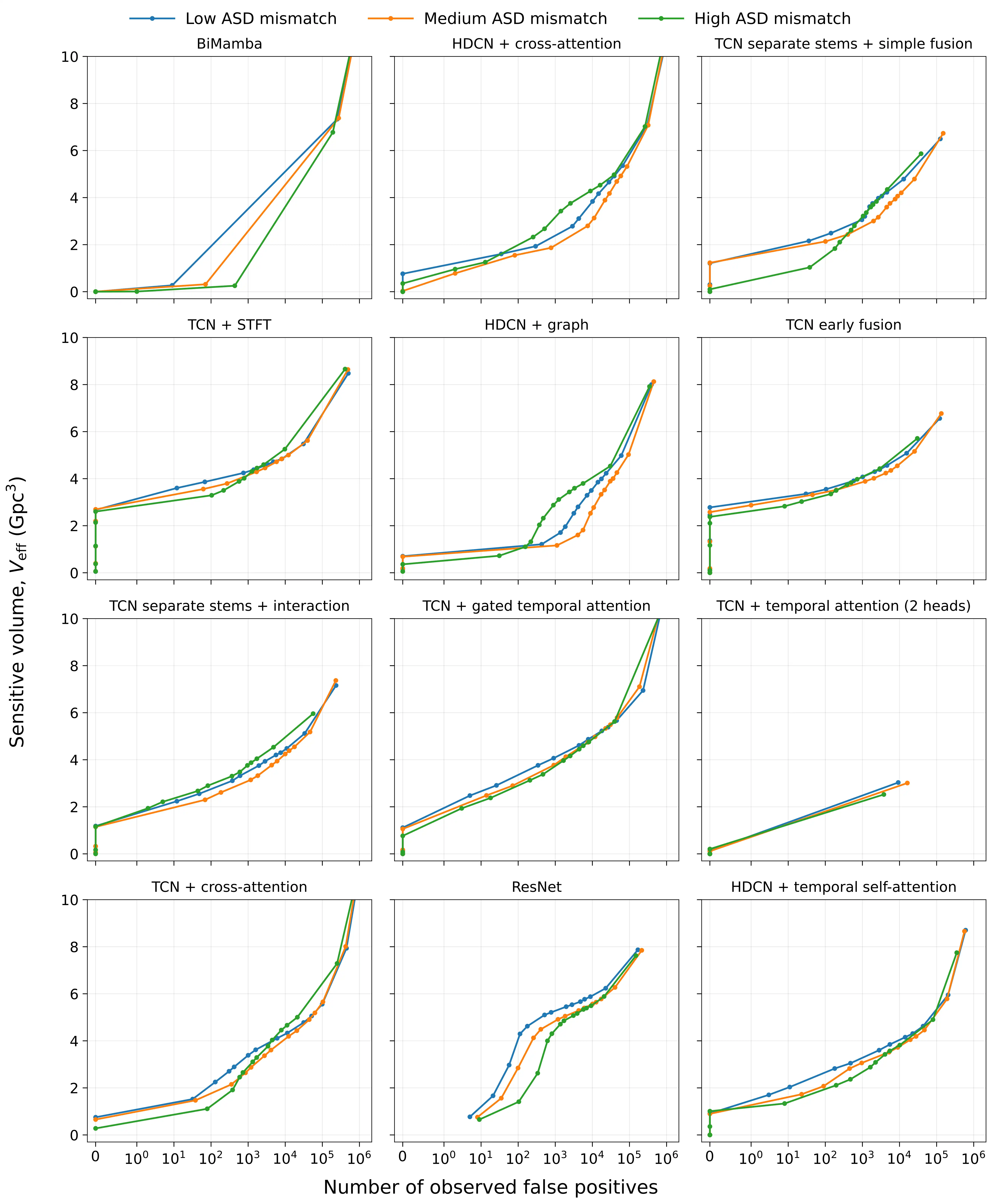
Comparison of lightweight neural gravitational-wave detector architectures across different levels of detector-noise mismatch.

Figure 2. Comparison of twelve architectures on held-out O3a data, split by how closely the evaluation noise matches the training noise. Each curve uses 2 weeks of effective background lifetime.

Final Results:

After selecting the architecture and pipeline on O3a data, I froze the setup and evaluated four independently trained models on a held-out O3b interval from January 28 to February 29, 2020. This contains 22.7 days of coincident Hanford–Livingston data and 13 confident GWTC-3 events.

At the threshold chosen on O3a data, the four models recover 8, 9, 9, and 9 of the 13 events, with 0, 0, 1, and 0 false-positive triggers. For comparison, we considered Tian et al's published benchmark on the same stretch of O3b time, developed within our group. Their benchmark produced hundreds to roughly 1,000 false-positive triggers, recovering 6 events. Our results are single-model results: there is no ensemble coincidence, external glitch veto, spectrogram review, or manual removal of triggers. This distinguishes the model from several established, high-performing pipelines that rely on additional coincidence, veto, or post-trigger processing stages for similar real-event performance. Such comparisons are discussed in more detail in Section 3.2.2 of the paper . Eight events are recovered by every training seed, and a ninth is recovered by three of the four.

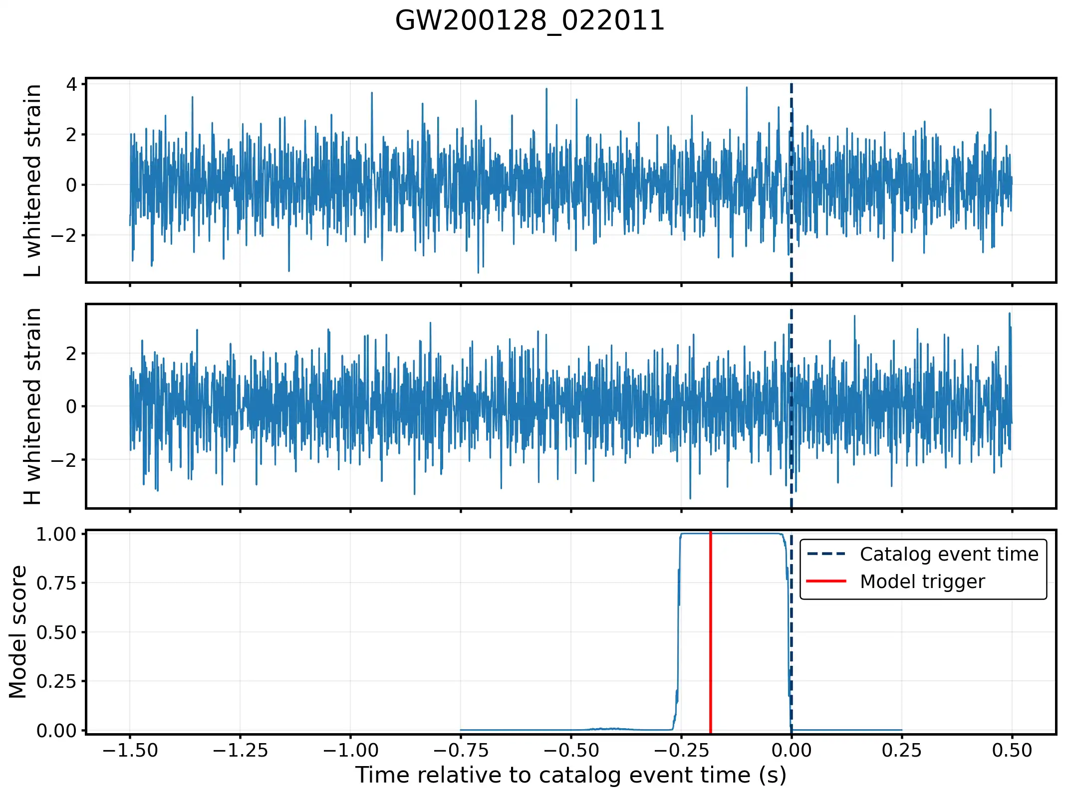
Recovery of gravitational-wave event GW200128_022011 using the final early-fusion TCN.

Figure 3. Example recovery of GW200128_022011. The upper panels show whitened Livingston and Hanford strain and the lower panel shows the model output around the catalogued merger time.

To measure the background beyond what is possible from a single month of data, I also evaluated each training seed on 365 days of effective O3b noise together with 10,000 BBH injections. At the operating threshold used for the real-event test, the median sensitive volume is 5.40 Gpc³ at a median false-alarm rate of 20.5 yr⁻¹. At a stricter threshold, three of the four models produce no false alarms in a year of background and the fourth produces one, while retaining a median sensitive volume of 4.55 Gpc³.

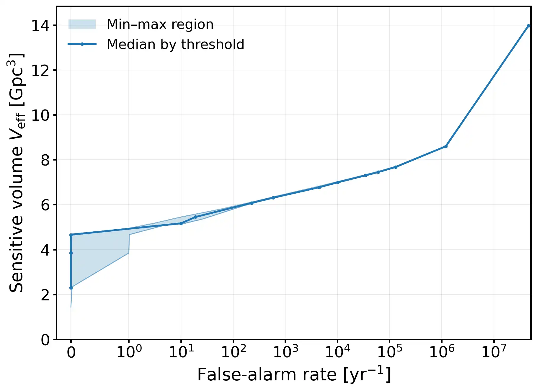
Sensitive volume versus false-alarm rate for four independently trained gravitational-wave detection models.

Figure 4. Sensitive volume versus false-alarm rate from the year-scale O3b injection study. The curve shows the median across four independent training runs and the shaded region shows the seed-to-seed range.

Software:

The final TCN model has about 116,000 trainable parameters and runs roughly 100 times faster than real time on a single A100 GPU. The public repository includes the full workflow for downloading GWOSC data, constructing injections, training different architectures, running continuous inference, generating triggers, and evaluating sensitivity and false-alarm rates. The configurations and checkpoints used for the final O3b analysis are also included.